

In short
- Accidentals scale with the window. In any entangled photon source lab, two uncorrelated detectors produce A = N₁·N₂·Δt false coincidences per second. At 400 k and 350 k counts/s and a 1 ns window that is 140 per second.
- CAR falls as brightness rises. With low dark counts the coincidence-to-accidental ratio is roughly 1/(R·Δt). Five million pairs per second in a 1 ns window give a CAR of about 200.
- Size the window from the jitter. A window of about 2.2 × the combined timing jitter (FWHM) keeps 99 % of the true pairs. A wider window only adds accidentals.
- Heralding efficiency shows the losses. C/N₂ and C/N₁ give the end-to-end efficiency of each arm, including coupling, filters and detector efficiency.
Every measurement in an entangled photon source lab ends with two detectors, a timing unit and a number: coincidences per second. Visibility, Bell parameters, heralded purity and tomography are all built on it. This review collects the relations used in current practice and the lessons of recent work on pair sources, with a worked example and a calculator.
What coincidence counting measures
A spontaneous parametric down-conversion (SPDC) source emits signal and idler photons within a few picoseconds of each other. The electronics time-stamp every detection, and a coincidence is counted when detections in arm 1 and arm 2 fall within a window Δt around the expected delay.
A run is described by the singles rates N₁ and N₂ and the coincidence rate C. Singles include photons whose partner was lost, dark counts and stray light. Coincidences include true pairs and accidentals: unrelated detections that happen to share the window.
In a histogram of t₂ − t₁, true pairs form a narrow peak whose width is the system timing jitter, and accidentals form a flat floor. The goal is to keep the peak inside the window and the floor under it small.
The detection chain: detectors, timing and time tagging
Typical published ranges for the detector families used in pair-source labs are below. Values vary by model and wavelength; treat them as a starting point.
| Detector family | Typical band | Detection efficiency | Timing jitter (FWHM) | Dark counts | Dead time |
|---|---|---|---|---|---|
| Free-running single-photon avalanche diode (SPAD) | Visible to about 1 µm | About 50–70 % near 600–800 nm | About 300–600 ps (thin-junction types 30–60 ps) | Tens to hundreds of counts/s | About 20–50 ns |
| Gated telecom avalanche detector | About 1–1.6 µm | About 10–30 % | About 100–300 ps | Per gate; afterpulsing limits the rate | Microseconds hold-off typical |
| Superconducting nanowire detector (SNSPD) | UV to mid-IR, optimised per band | Above 85 % at the design wavelength | About 15–60 ps | Below 100 counts/s | About 10–50 ns recovery; needs a cryostat |
A modern time tagger adds a few to a few tens of picoseconds of jitter. Unlike fixed hardware coincidence logic, time tagging stores every time stamp, so the window, delay and accidental estimate can be chosen after the run, which makes it the better choice for development.
Accidental coincidences and the CAR
For independent detectors, a detection in arm 1 finds an unrelated arm-2 detection inside a window of full width Δt with probability N₂·Δt, so
A = N₁ · N₂ · Δt
N₁ and N₂ are the total measured rates, dark counts included. The quality figure used across the literature is the coincidence-to-accidental ratio:
CAR = (C − A) / A
Some papers use C/A, larger by one. Writing the singles in terms of the pair rate R and the arm efficiencies η₁ and η₂: N₁ = R·η₁ + D₁, N₂ = R·η₂ + D₂, and C − A = f·R·η₁·η₂ (f = share of true pairs inside the window), with small dark counts:
CAR ≈ f / (R · Δt)
The efficiencies cancel: CAR depends on how many pairs you generate per window. Better detectors raise the coincidence rate but not CAR; a narrower window or a lower pair rate does.
Accidentals also cap visibility: with a perfect state the minimum reading is the floor A, so visibility is at most CAR/(CAR + 2). A CHSH Bell test needs a visibility above 1/√2 ≈ 0.707, which requires a CAR of at least 4.8 even before any other imperfection. Subtracting accidentals is fine for characterising a source if reported, but not in a test that claims to close loopholes.
Choosing the coincidence window
The true-pair peak in the time-difference histogram has a width set by the jitter of both detectors and the electronics. For approximately Gaussian contributions, the widths add in quadrature:
FWHMsys = √(j₁² + j₂² + je²) f = erf(Δt / (2√2 · σ)), with σ = FWHMsys / 2.355
A window of 1.66 × FWHMsys keeps 95 % of the true pairs and 2.19 × FWHMsys keeps 99 %. Beyond that, the window only collects accidentals. Example: two 350 ps SPADs and 20 ps electronics (FWHMsys = 495 ps), singles 400 k and 350 k /s, 28 355 true pairs /s.
| Window Δt | True pairs captured | True coincidences /s | Accidentals /s | CAR |
|---|---|---|---|---|
| 0.25 ns | 44.8 % | 12 692 | 35 | 363 |
| 0.5 ns | 76.5 % | 21 701 | 70 | 310 |
| 1 ns | 98.3 % | 27 860 | 140 | 199 |
| 2 ns | ≈ 100 % | 28 355 | 280 | 101 |
| 5 ns | ≈ 100 % | 28 355 | 700 | 41 |
A narrow window improves CAR but discards real pairs and understates heralding efficiency. For characterisation, capture 95–99 % of the peak. Faster detectors move the whole table: with 50 ps detectors the same 99 % capture needs a window of only about 0.16 ns, and accidentals fall by a factor of about seven.
Heralding efficiency and the pair rate
Because pairs are born together, the ratio of coincidences to singles gives the efficiency of the other arm without a calibrated reference, the classic absolute-calibration method for SPDC sources:
η₁ = (C − A) / (N₂ − D₂) η₂ = (C − A) / (N₁ − D₁) R = (N₁ − D₁)(N₂ − D₂) / (C − A)
η₁ is the probability of detecting the arm-1 photon given its partner was detected. It includes mode overlap, fiber coupling, filters and detector efficiency. Low values usually mean a spatial-mode problem: pump focus, collection waists or crystal angle are not matched. R is the pair rate at the source.
Detection-loophole-free Bell tests need more than 2/3 end-to-end efficiency per arm. Most teaching and development set-ups operate at 5–30 %, limited by coupling optics, not detectors.
Brightness versus purity: the pump-power trade-off
More pump power raises coincidences linearly but accidentals as R². Arm efficiencies 7 % and 8 %, 500 dark counts/s, 1 ns window (98.3 % capture):
| Pair rate R | Singles N₁ / N₂ | True coincidences /s | Accidentals /s | CAR |
|---|---|---|---|---|
| 10⁵ /s | 7.5 k / 8.5 k | 550 | 0.06 | ≈ 8 600 |
| 10⁶ /s | 70.5 k / 80.5 k | 5 505 | 5.7 | ≈ 970 |
| 5 × 10⁶ /s | 350 k / 400 k | 27 524 | 140 | ≈ 196 |
| 2 × 10⁷ /s | 1.4 M / 1.6 M | 110 096 | 2 242 | ≈ 49 |
Compare sources at the same coincidence rate or R·Δt, not at their best CAR. At the highest rates check dead time too: at 1.6 M counts/s a 50 ns dead time hides about 7 % of detections, unequally in the two arms.
Worked example: reading a coincidence measurement
A polarisation-entangled source pumped at 405 nm sends 810 nm photons into two fibers and two SPADs with 350 ps jitter, 500 dark counts per second and 50 ns dead time. The time tagger adds 20 ps. The run gives N₁ = 400 000 /s, N₂ = 350 000 /s and C = 28 000 /s in a 1 ns window.
- Accidentals: A = 400 000 × 350 000 × 1 × 10⁻⁹ = 140 /s, so C − A = 27 860 /s.
- CAR: 27 860 / 140 = 199. The visibility ceiling from accidentals alone is 199/201 = 0.990, well above the CHSH threshold of 0.707.
- Heralding efficiencies: η₁ = 27 860 / 349 500 = 7.97 % and η₂ = 27 860 / 399 500 = 6.97 %.
- Pair rate: R = 399 500 × 349 500 / 27 860 ≈ 5.0 × 10⁶ pairs/s.
- Window check: FWHMsys = √(350² + 350² + 20²) = 495 ps. The 1 ns window captures 98.3 % of the true pairs; 99 % needs 1.08 ns.
- Dead time: at 400 000 /s and 50 ns, about 2 % of detections are lost. Acceptable, but it will not stay negligible if the pump is doubled.
Verdict: bright and clean, but with 50–70 % detector efficiency at 810 nm, 7–8 % heralding efficiency points to the collection optics. The next step is mode matching and crystal alignment, not new detectors.
Coincidence calculator: accidentals, CAR and heralding efficiency
Enter the rates from your time tagger and the detector data to get accidentals, CAR, heralding efficiencies, pair rate, window capture and dead-time loss.
Assumes independent detectors with Poisson statistics, Gaussian timing jitter and a window centred on the true-pair peak. CAR is defined as (C − A)/A. Heralding efficiencies are not corrected for the window capture fraction or dead time; divide by the capture fraction if your window is narrower than the peak.
Setting up coincidence counting in an entangled photon source lab
- Find the delay before you set the window. Record a ±100 ns histogram and locate the peak. Coax (velocity factor 0.66) adds about 5.05 ns/m, silica fiber about 4.9 ns/m; re-measure after any cable change.
- Measure accidentals, do not only calculate them. Read the histogram floor away from the peak. If it is well above N₁·N₂·Δt, look for afterpulsing, pump leakage or reflections.
- Block the pump and record dark and background counts with the room lighting used in the run.
- Keep the detectors in their linear range. Above a few per cent N·τdead, reduce pump power or correct.
- Optimise the source, not the numbers. Profile the pump beam at the crystal, keep the crystal within its angular acceptance, and adjust tip, tilt and position independently.
- Report the full set: window, delay, singles, raw coincidences, accidentals and how they were obtained, CAR definition, and whether accidentals were subtracted.
What recent work shows
Three trends stand out. Integrated and waveguide sources report CAR above 10 000 at low pump power with heralded g⁽²⁾(0) below 0.01, and fiber-pigtailed telecom sources are becoming practical lab tools. Heralding efficiency is now the headline figure: careful mode matching plus superconducting detectors has pushed it above 80 % in bulk sources. Time-resolved analysis of the full time-tag record is used to separate true pairs from background and multi-pair events.
The lesson: brightness alone is not a specification. Quote coincidence rate, CAR and heralding efficiency together, at a stated pump power and window. The relations here are standard quantum-optics material; our engineers can share derivations and literature on request. For the physics of entanglement and correlation curves, see Understanding photon entanglement, and for phase matching and SPDC see Introduction to nonlinear optics and its quantum impact.
IZAK products for this application
Coincidence numbers are only as good as the crystal and pump alignment.
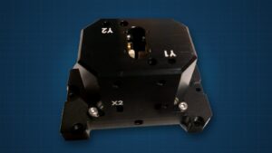
 Nonlinear crystal mountQuantumAlign NLO Kinematic StageX/Y ±2 mm and lockable tip/tilt for SPDC and SHG crystals, single or two crossed crystals on one axis, with an optional 40–70 °C oven held within ±0.3 °C.View product →
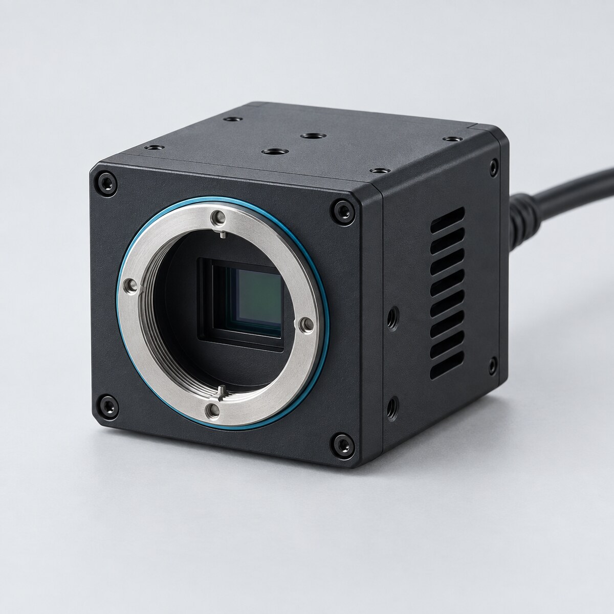 Beam profilingUV–VIS–NIR Laser Beam ProfilersMeasure the pump spot at the crystal and the collection-mode waists, 300–1100 nm, with ISO 11146 second-moment widths.View product →
For a complete entangled-photon source or a teaching-lab set-up built to your specification, see custom electro-optical system design.
Frequently asked questions
QHow do I calculate accidental coincidences?
QWhat coincidence window should I use?
QWhat is a good CAR for an entangled photon source?
Tzachi Sabati
CEO, IZAK Scientific
Physicist specializing in photonics and quantum technologies, with deep expertise in quantum sensors and advanced optical systems. Leads the Advanced Quantum Lab course at the Technion, bridging academic excellence with industry innovation. At IZAK Scientific, provides cutting-edge photonics-based solutions, developing customized inspection and sensing systems for R&D and production. Passionate about advancing quantum sensing applications and integrating novel technologies to meet industry needs.
Get new IZAK guides and tools by email
One short email a month: new technical articles, free calculators and product updates in laser measurement and electro-optics. No spam, unsubscribe anytime.
